While it is well-known that log data can be used to constrain prestack depth migration (PSDM) model building, it is much less-appreciated that machine-learning (ML) can be leveraged to augment the value of the well data for this important seismic imaging task. In this talk we will show how ML-predicted sonic data can be used to improve the PSDM velocity model building process.
ML algorithms allow the estimation of missing well-log information by training a network to predict the absent curve from a combination of one or more other measured curves. We have performed regional-scale estimations of such missing well data for several onshore unconventional US basins, including the Delaware Basin, which is the focus of the present study. Among the various tracks predicted by this so-called “ARLAS” process (“Analytics-Ready LAS”), sonic curves are estimated over most of the length of the wellbore, resulting in a very large database of velocity information that can be utilized for geological purposes, with PSDM model-building being one of the main applications. Accordingly, a test was performed on the TGS West Lindsey 3D survey in which the PSDM image obtained from a traditional model-building approach (i.e., using measured sonic information) was carefully compared against the image obtained from an approach using both measured and ARLAS sonic information. The West Lindsey 3D is a suitable candidate for such a test because it straddles the Grisham fault, a major feature active in the late Mississippian which has imparted over 2000 ft of throw to the deep basement structure (Figure 1), resulting in considerable geological complexity.
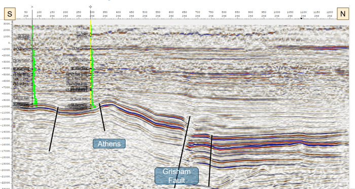 Figure 1 – Cross section extracted from the 3D dataset with the Grisham Fault annotated
During the data mining process, we found 13 wells with valid measured sonic extending from shallow to deep, and an additional 10 wells with ARLAS-predicted sonic logs within the 3D outline. Figure 2 displays the distribution of the measured and ARLAS sonic logs within the 3D outline and associated cross-section. Note, this cross section is not at scale and all wells are displayed within equal distance. The addition of the ARLAS sonics is important as many of those predicted curves fall within areas which lack existing measured sonic support. For example, the purple ARLAS well numbered “7” in the LHS pane of Figure 2 resides just north of the Grisham fault, and is notably distant from any wells containing measured sonic data (i.e., there are no nearby yellow dots); we would therefore expect this ARLAS well to impose useful geological control on the PSDM velocity model construction.
Figure 3 shows two velocity cubes, one constructed using both ARLAS and measured sonic information (Figure 3a), and the other constructed using only measured sonic information (Figure 3b). Note the increased lateral variation at depth across the Grisham fault in the “with-ARLAS” cube in Figure 3a compared to its “non-ARLAS” counterpart in Figure 3b; in particular the faster (hotter colors) velocities on the downthrown side of the fault (white ellipse, Figure 3a) are consistent with geological expectation.
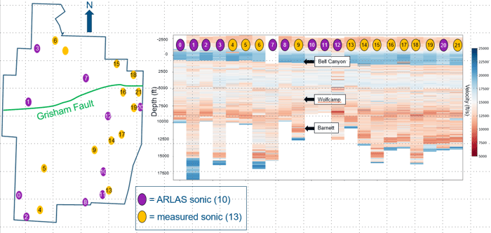 Figure 2 – Location of measured and ML-estimated sonic logs and cross section of sonic log data.
Two anisotropic PSDMs were performed: first, a “with-ARLAS” migration using the vertical velocity field shown in Figure 3a, and second, a “without-ARLAS” migration using the vertical velocity field shown in Figure 3b.
Figures 4a (“with-ARLAS”) and 4b (“without-ARLAS”) show the depth-mistie at the deep Barnett level for the two PSDM results. South of the Grisham fault, where there is a relative abundance of measured sonic information, the mismatch (i.e, contoured difference between well tops and interpreted PSDM horizon) is very similar between the two PSDM outputs. However, north of the Grisham Fault, the mistie is clearly superior (i.e, smaller) for the “with-ARLAS” result in Figure 4a, an observation which is consistent with our hypothesis that the injection of ARLAS sonic information in the vicinity of the Grisham Fault is providing a more geologically realistic velocity model.
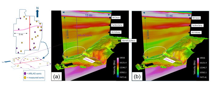 Figure 3 – Two PSDM velocity cubes. (a) cube created with both measured and ARLAS sonic information; (b) cube created with only measured sonic information.
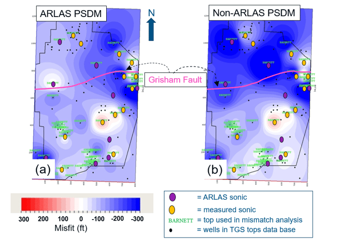
Figure 4 – Top-to-seismic depth-mistie maps at Barnett Shale level. (a) PSDM using “with-ARLAS” velocity model; (b) PSDM using “without-ARLAS” velocity model.
We are very encouraged by the above results and are motivated to take next steps towards commercial deploy. Such steps include implementing an interpolation algorithm capable of infilling missing vertical segments of ARLAS sonic tracks (a step which would waive the requirement of needing vertically contiguous ARLAS coverage from shallow-to-deep, allowing us to use much more ARLAS information than we have used in the present study) and also a mechanism to gauge reliability of the ARLAS predictions by considering confidence-interval curves which are automatically generated by the machine-learning process. Whatever the final form of our production offering, we are currently reveling in our confirmation here that machine-learning can indeed enhance the value of information associated with well data in PSDM model building!