
| TGS insights give you the stories behind Energy data. These regular short reads feature thought provoking content to illustrate the use of Energy data in providing insight, nurturing innovation and achieving success. |
Could geothermal energy be developed from existing oil and gas wells? This question is currently drawing a lot of industry attention. If one can use existing wells for geothermal installation, it could dramatically accelerate geothermal energy development worldwide. There are several ways to produce geothermal energy from oil and gas wells; one involves converting a well from producing oil and gas to producing geothermal. Another way is to coproduce several sources of energy from a well: oil and heat. Many factors must be considered before such an undertaking, and not all existing wells are up to the task.
Huge Data Availability
There is a vast resource of data and analyses utilized by the oil and gas industry that may be effectively repurposed for other industries, such as developing geothermal resources. This data serves as a common resource for both the oil and gas and geothermal energy communities to explore and evaluate investment opportunities. Examples include:
- Oil and gas well performance/production data:
- Decline curve analysis
a. Forecast economic limit – end of economic life
b. Maximum produced fluid per month – oil, water, and sum (average max daily rate) - Well completion data
c. Completed zones, perforated intervals (depth, formation)
d. Casing diameters
e. Completion histories
- Decline curve analysis
- Basin temperature data and models
- Gradient-based corrected subsurface formation temperatures
- Gradient-based corrected subsurface formation temperatures
Decline curve analysis on well production data is integral to the economics of the oil and gas industry. Among many uses, production forecasts provide recoverable reserve estimates and input to the future value of wells. The economic limit of a well is reached when the produced resources’ net value drops below the well operating cost. Decline rates of multiple wells contribute to field reserves analyses and operational investment planning.
 |
New Energy Update e-FeedSubscribe to our free daily e-newsletter providing you with the latest news in wind, solar, geothermal and CCS. Capture the key events associated with the world's Energy Transition, collating headlines from multiple sources to provide an easy-to-consume daily email briefing. |
Identifying End-of-Life Potential
Economic limits of wells (end-of-life) data can be leveraged by many businesses, including the geothermal community, where the repurposing of aging wells is being considered. Forecasted economic limits can vary with commodity price and operator efficiency, affecting decisions on well re-completion, shut-in, and abandonment, with lease restoration and other liabilities. However, having a large standardized dataset with shut-in timeframes can be useful in prospecting and planning for future uses, including the geothermal resources still untapped.
Figure 1 illustrates two examples of forecasted economic limits in decline curves. The upper illustration shows a well that has been in production for over 50 years, with the potential to continue production for another five years. The lower image shows a well with a rapid decline rate that may be a shut-in candidate within two years.
Decline curves are also referenced for comparative analysis of potential fluid flow rates in the evaluation of repurposing.
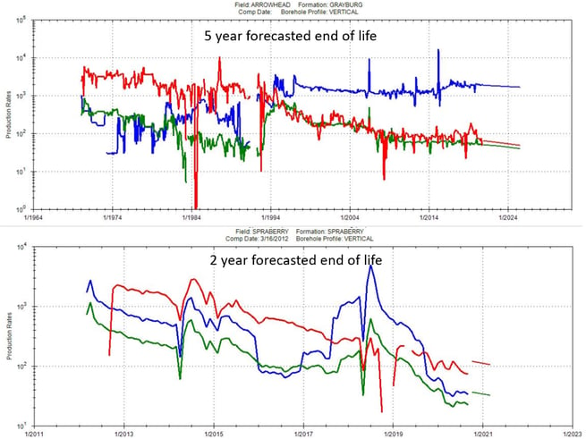
Figure 1: Decline curves used to forecast end of life. Red=gas, green=oil, blue=water. The straight sloping line at the right of each plot shows the forecasted end of economic production.
Combining end of life economic data with well depth, producing formations, completion intervals, and maximum production rates within a stratigraphic framework offers value to companies interested in assessing alternatives to abandoning their assets.
The images in Figure 2 illustrate how the forecast end-of-life data can be parsed to highlight various trends. The large image shows a subset of the forecast end of economic life for the Silurian and Ordovician formations, the oldest producing zones in the Delaware Basin, and aside from the basin flanks, usually the deepest. The well spot colors represent the remaining expected economic life of 10 years, five years, one year, and wells presently shut-in.
The inset in Figure 2 shows forecasted economic limits for well locations in the Permian Basin with drilled vertical depths of >10,000 ft. The density of wells with ten-year forecasts indicates newer development in the Midland and Delaware Basin centers, and trends of shut-in and wells in the last stage of decline are more evident on the basin margins
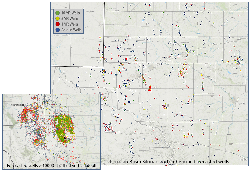
Figure 2. Wells in the Permian Basin, drilled to the Silurian and Ordovician formations with forecasted economic limits of 10, 5, 1 yr and shut- in are shown on the large map. Production from the Silurian and Ordovician is primarily gas and gas liquids. The inset map shows al wells with >10,000 ft drilled vertical depth with the same forecast color legend
Evaluating Key Trends
TOne of the tools useful in an oil and gas trend evaluation is the maximum fluid flow rate, which is an indicator of attractive reservoir properties, especially where clusters of wells exhibit similar flow characteristics. This same tool can be used to review clusters of wells to convert to geothermal production at the same time to improve project performance. Thus, individually an oil and gas well considered for repurposing to geothermal energy may not individually meet the high flow rates required for a geothermal project. However, in clusters, they may be more than adequate. The image in Figure 3 shows a map view of the Permian Basin area with shut-in wells that have exceeded 2000 bpd (barrels per day) combined as oil and water at some point in their production history. The subset has further been culled to wells with a 4 inch or greater minimum production casing diameter. The largest casings are more appropriate for geothermal fluid extraction.
The graph on the right in Figure 3 shows a different view of the data with the forecast well subset of 5 years economic limit. The vertical axis is minimum casing/liner diameter, and the horizontal shows the maximum combined oil and water volume month. Note that for this data subset, the average monthly fluid volumes rarely exceed 1,000 bpd, yet there are a number of exceptions, with some wells producing over 10,000 bpd.
The use of the fluids as a geothermal resource vary with the amount of fluids necessary for project economic success. Typically, higher temperatures (> 275°F) with high flow rates (>10,000 bls/day) are appropriate for electrical production on-site and if combined with other heat sources (compressors, solar, etc.) sold off-site. As either the resource flow rate or temperature decreases, projects considered for moderate use are generally either on-site or within a 6-mile radius. These include direct use (or even deep direct use) for agriculture or industry, small electrical production, and district or building heating and cooling. Production of the fluid is also a geochemical extraction opportunity if the additional infrastructure is added.
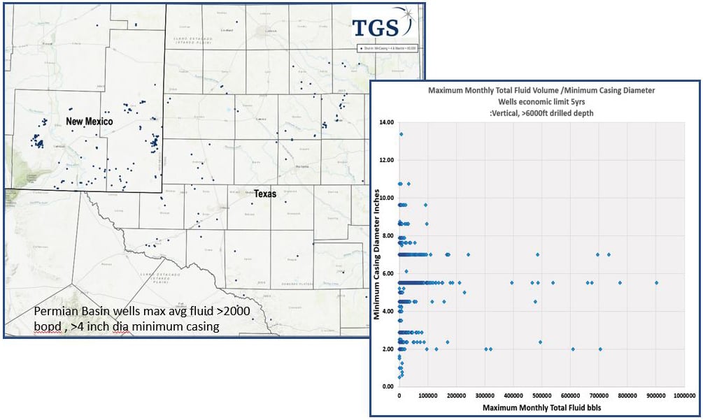
Figure 3. The map shows shut-in wells between 6000 and 10,000 ft drilled depth with over 2000 bpd average daily fluid production rate, and at least 4 inch minimum casing diameter. The inset graph shows wells with 5 year end of life forecast, with minimum casing diameter on the vertical axis and the maximum fluid volume (monthly) on the horizontal axis.
Basin Structure and Temperature Models
Basin stratigraphy and structure and basin temperature models yield additional relationships that can enhance perspective. Figure 4 below displays the Delaware Basin portion of the well-set (shown above in Figure 2) as an overlay on a 10,000 ft depth slice of a Delaware Basin temperature model. The corrected temperature data shown were extracted from a 3D volume that used over 5,000 wells with bottom hole temperatures along with proprietary formation tops for the stratigraphic framework. The model cell size is 50 ft vertical x 2,500 ft horizontal, providing corrected temperature data for the entire sedimentary section from ‘basement’ to surface.
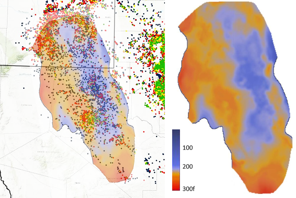
Figure 4.The left image shows a horizontal slice of the basin temperature model at 10000ft depth with an overlay of the forecasted end of life for wells (from Figure 3) with total drilled vertical depths greater than 10,000 ft. The image at right shows the temperature slice alone for reference. The color bar is set to visually enhance the temperature differences at the 10,000 ft depth. The formation temperatures at this depth range from 200 °F to 280 °F. The line on the right image shows the location of the vertical section in Figure 5
Significantly, the model’s corrected temperatures at 10,000 ft depth vary laterally from roughly 200 °F to 280 °F. This temperature is in the intermediate range of extractive geothermal energy per the USGS resource depiction. The images illustrate the comparative perspective at basin scale using multiple datasets. The data can be accessed as cloud-based interactive layers for rapid scanning of convergence of attributes.
Lateral variations in formation temperatures across the depth slice imply influences of structural and basement sources of higher heat contribution. Figure 5 is a perspective view of N-S section of the basin temperature model over the entire Delaware Basin
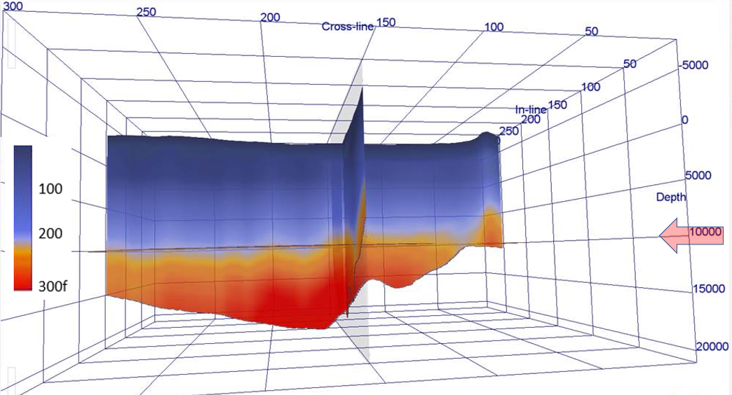
Figure 5. N-S cross-section perspective of the Delaware Basin temperature model. The model includes the full sedimentary section with temperatures ranging to over 300 °F at ‘basement’ to the upper surface at ground level. The image is rendered in OpendTect software.
Co-Rendering Spatial Data
Additional analysis tools are available with large datasets that can be easily referenced to the library of available spatial data. One example is the co-rendering of well forecast data (accessible by depth and/or formation) along with stratigraphic, structural, and lithologic information.
Although much of the focus on geothermal resources is for electrical production, the direct use of heat itself is expected to grow in the US, as it has done in other global regions. These data requirements are for shallower depths (< 10,000 ft) and temperatures lower than 300 °F, yet more typically below 200°F. In this example (Figure 6) we show the forecast economic limit of wells with drilled depth > 6,000 ft. The model temperature at this depth ranges from roughly 150 °F to 240 °F with temperatures in the basin center varying from 160 °F to 210 °F over relatively short distances (~6 miles ). Combining these slices within the basin with the additional information regarding agricultural and manufacturing heat demand as a layer (Figure 6) can be used to forecast end-of-life wells used locally as an additional resource.
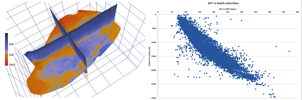
Figure 6. Basin temperature model perspective view with depth slice at 6000 ft. The temperatures at 6000 ft range from roughly 150 °F to 240 °F. The raw borehole data, as input to the corrected temperature model, are shown on the right image.
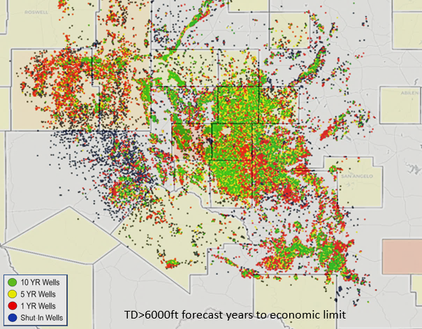
Figure 7. National Renewable Energy Laboratory (NREL) layers; Manufacturing heat demand in pale orange and agricultural heat demand in yellow, by county, overlain on forecast economic limit groups of wells drilled to 6000 ft or deeper.
In Conclusion
The use of existing TGS data, analysis, and available tools provides resource exploration opportunities for both the oil and gas and geothermal communities. As the two industries work together to find economical methods to develop geothermal resources within the sedimentary basin, all aspects of the energy industry stand to grow.
With thanks to James Keay (TGS), Maria Richard (SMU), Matt Mayer (TGS), Alejandro Valenciano (TGS), Katja Akentieva (TGS).