Imaging and Processing
To meet the challenges of today's quest for hydrocarbons, our research and development professionals are continually developing new technology and workflows for seismic imaging, as well as enhancing existing ones. We have the technology, expertise and resources to exceed the highest geophysical processing objectives powered by our proprietary Imaging AnyWare® imaging software.
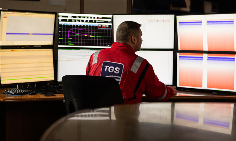
The TGS Energy Data Value Chain
TGS is rethinking the traditional service model by integrating Geophysical Modelling, Acquisition, Processing & Imaging and Discovery into an accelerated cycle of insight, driving impact across the energy data value chain.
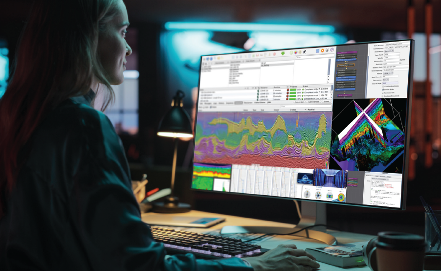
Imaging AnyWare® Software
Imaging AnyWare® is a versatile, user-friendly software that excels in both cloud and on-premises environments, efficiently handling extensive datasets across global geological basins. Its modern architecture and advanced geophysical algorithms enhance operational efficiency, supporting various acquisition types and incorporating techniques in signal processing, imaging and machine learning. With an intuitive user experience and powerful QC tools, it enables seamless collaboration and rapid solution development.

Geoscience Innovation Powered by People
At TGS, every imaging and processing project is built on a strong foundation of geoscience expertise and driven by the passion of our people. Our teams combine deep domain knowledge with technology to deliver insights that empower exploration and development decisions. From project planning to advanced imaging and geological interpretation, we focus on precision, innovation and collaboration.
Learn more about the science and stories behind our work, where our experts share the thinking that shapes each solution.
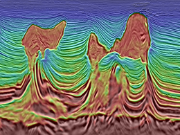
Full Waveform Inversion (FWI)
By using the full seismic wavefield, FWI enables precise reconstruction of complex subsurface structures, improving depth migration and reservoir characterization.
.png?width=1256&height=752&name=TGS_website_Broadband_Processing%20(2).png)
Subsurface Imaging Solutions
Broadband processing and high-end seismic imaging methods tailored to deliver a broader frequency spectrum in the recorded signal for clearer and more detailed final images.
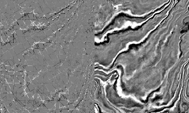
2Dcubed
2Dcubed is a structurally conformable interpolation engine that matches 2D data and uses it to create a 3D volume that is interpretable on a regional scale.
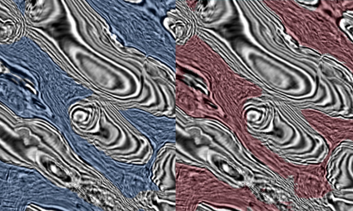
Machine Learning (ML)/AI
AI-integrated imaging workflows and foundational ML models trained on the most extensive geosciences data library in the energy industry.
Speak to a Specialist
Interested in a live data review or demo? Let us know your needs and we’ll connect you to the right person or team.
Book a Data Viewing
Want to see the latest seismic data solutions and imaging technologies in your region of interest or for the next license round? Book a data viewing with one of our experts.
Discuss Your Seismic Data Needs
Every need is different and we'd like the opportunity to discuss yours further. Speak to one of our data or geoscience experts to customize seismic solutions specific to your requirements.
