Wireline logs are a fundamental aspect of subsurface property characterization. However, economic constraints often limit data acquisition from specific logs or depth intervals, resulting in incomplete information from the well’s surface to its base in many areas. An alternative that addresses the lack of data is to create synthetic curves. With the advent of data science and the availability of digitized well data, machine learning (ML) algorithms can be used to predict missing logs or log intervals. TGS’ Analytics Ready LAS (ARLAS) leverages both the vast amount of well log data in the TGS library as well as data management infrastructure. TGS algorithms provide curve predictions for five standard curves, including the confidence intervals of each log which can be used for automated interpretation such as facies classification or basin stratigraphy.
TGS has developed an end-to-end ML workflow for well-log prediction at a basin scale. The workflow starts with the well-log cleaning process, which involves extensive data cleanup before ML training and inference. After the well logs have been cleaned, the workflow consists of ML training, validation, and inference based on a gradient-boosted regression trees algorithm. The ML models have been created across all the US unconventional onshore basins (Figure 1).
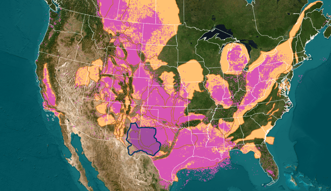
Figure 1. US onshore basins with existing ARLAS ML models for predicting missing data in well logs. The dark blue polygon encircles the data used for the Permian Basin model.
Before training ML algorithms, data preparation and cleanup are necessary. Traditional workflows require manual log cleanup on a per-well basis. Nonetheless, this manual approach needs to be more scalable for ML applications. To develop practical ML tools for well-log prediction, an automated pipeline for well-log cleaning is required. Our cleanup methodology includes processing steps such as curve categorization, unit standardization, log splicing, depth shifting, normalization, and inferior data removal or editing (Figure 2). Our design principle for this pipeline is to minimize the need for human interpretation and save time by automating complex processes. This approach enables basin-wide application and improves consistency and accuracy in decision-making.
.png?width=650&height=225&name=MicrosoftTeams-image%20(54).png)
Figure 2. TGS’ well log cleanup workflow.
The log-cleaning workflow begins with curve categorization, which defines curves based on measurement type, logging tool, and operator. In the ARLAS model, the curve categories include Total Gamma Ray, Neutron Porosity, Compressional Sonic, Bulk Density, and Deep Resistivity. The Neutron Porosity and Deep Resistivity curves are further classified based on rock matrix setup and penetration depth. By creating a comprehensive list of standardized curve mnemonics for each category, users can easily update the list when encountering new unknown mnemonics. The importance of curve mnemonics is exemplified in the Permian Basin, where the same mnemonics can be encountered for different log types.
After curve categorization, unit standardization is applied to all logs in a basin. This step corrects nonstandard units, typos, and mistakes. Figure 3 (a-b) presents the results of fixing the mnemonics and units of gamma ray logs for an arbitrary cross-section of 800 wells in the Permian Basin. The next step is log splicing, which combines similar curve measurements from different logging runs to construct a single curve. Log splicing involves selecting the primary and secondary curves in all available logging runs and calibrating them to ensure they are on a similar scale. The effects of splicing are shown in Figure 3 (c).
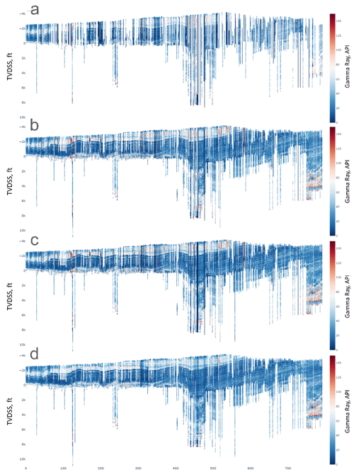
Figure 3. Change in the state of an arbitrary gamma ray cross-section in the Permian Basin during the cleanup workflow. Cross-section (a) shows data with basic mnemonics and unit analyses of common mnemonics and standard units. Cross-section (b) shows the same data after more rigorous mnemonic analyses, fixing mnemonic clashes, checking, and fixing unit issues. Due to thorough mnemonic and unit QC (Quality Control), several logs are added to the cross-section. Cross-section (c) shows the effect of log merging. The wells have better depth coverage. Cross-section (d) shows the impact of basin-scale log normalization. Artificially high and low gamma ray values present in (c) are fixed in (d).
The penultimate step is log curve basin-scale spatial normalization, which involves bringing logs of the same type from different wells to the same scale to have similar responses from similar rocks across the basin. This process is necessary because basin-scale well log datasets contain wells of different vintages, logging tool manufacturing, calibration variations, inconsistent log units, changes in the borehole environment, and various environmental corrections. Figure 4 shows the effect of spatial normalization on two adjacent wells. After normalization, the gamma ray log range is similar for both wells. Figure 3 (d) shows the effect of basin-scale log normalization on the Permian cross-section view.
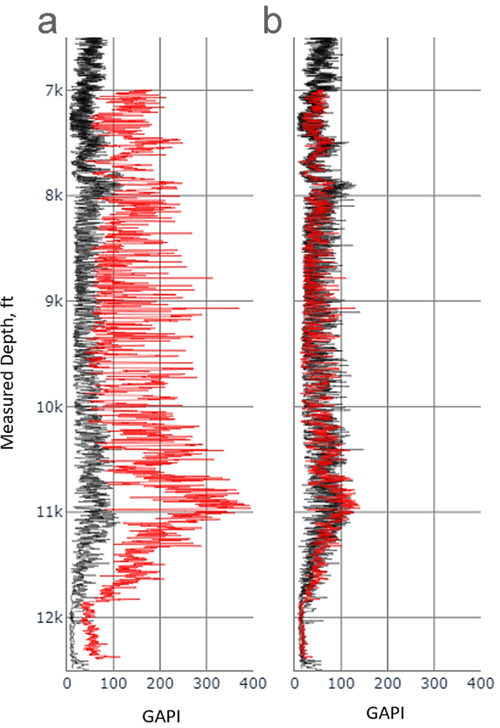
Figure 4. Gamma ray curve (red) before (a) and after (b) normalization flow as compared to the reference curve (black).
Finally, a basin-wide limit is set to flag questionable intervals and complimentary curves such as density and caliper. These erroneous values may be due to borehole or equipment-related errors and are challenging to identify with machine learning. The limit enables the automated detection of bad data quality. Well-log curves may contain erroneous values due to borehole or equipment-related errors, which can be challenging to identify with machine learning. To automate the detection of bad data quality, a basin-wide limit is set to flag questionable intervals and complimentary curves such as density and caliper.
ARLAS is a machine-learning pipeline that predicts missing logs at a basin scale. It specifically targets five types of logs, including density, gamma ray, neutron porosity, deep resistivity, and compressional sonic. The pipeline uses a combination of input features, such as compressional sonic and gamma ray logs, logarithms of deep resistivity and neutron porosity, cube of bulk density, and spatial locations, to make accurate predictions. For each target curve, separate models are trained from different combinations of available measured curves using the Light Gradient Boosting (LGB) Tree Algorithm. Gradient boosting is a tree-based method with the capacity for modeling data-driven piece-wise target-feature interactions. It predicts a target value by building weak prediction models where each model tries to predict the error left over by the previous model. The algorithm concentrates on the data that does not give a good result by weighing them higher as new learners are trained.
TGS trains models for different combinations of input features and target curves because variations in feature availability may exist in each well and for different depths within the same well. Models were built depending on the available data and combined with recorded logs to fill the existing data gaps and improve data coverage. Figure 5 shows an example of using ARLAS models to fill data gaps in the bulk density log for one of the wells in the Permian Basin. In Figure 6, we show the results of ARLAS modeling for a cross-section of 800 wells in the Permian Basin for compressional sonic. The contrast in prediction accuracy between cross-sections (b) and (c) highlights the significance of implementing an automated cleanup process before applying ML to log data on a basin scale. The prediction error was calculated in a blind test comprising 679 wells, and the model's performance was evaluated in intervals where both data and prediction exist. The results show that ARLAS effectively predicts missing logs and improves data coverage, achieving a prediction quality of 90% to 95% if trained on clean data.
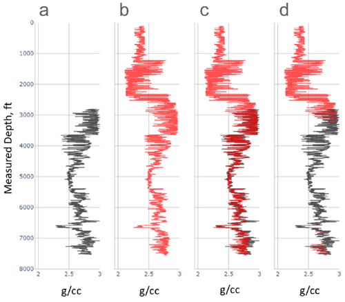
Figure 5. Application of the ARLAS modeling workflow for a bulk density log of one of the wells in the Permian Basin. The first track (a) shows the recorded data in the well (black). The second track (b) displays the ARLAS prediction (red). The third track (c) shows the measured data (black) and predictions (red). The fourth track (d) shows the final product, where the original data (black) is combined with the predictions (red) to extend the log depth coverage and fill data gaps.
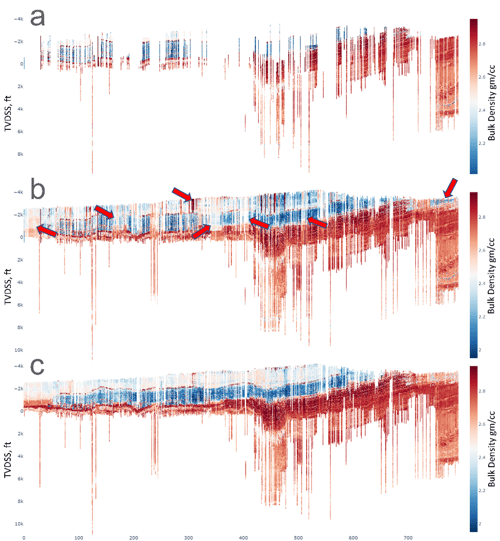
Figure 6. ARLAS modeling for a compressional sonic cross-section of eight hundred wells in the Permian Basin. Cross-section (a) shows the original measured data available in input LAS files without processing. Cross-section (b) shows the same cross-section with ARLAS predictions added to the original input data from (a). Cross-section (c) shows the improvements in ARLAS predictions using the cleaned input data. Red arrows indicate areas of most improvement.
We have demonstrated the importance of data cleaning in predicting well logs using ML algorithms, resulting in higher-quality outcomes on a basin scale. Our data-cleaning pipeline builds on our extensive data management infrastructure and is straightforward, fast, and requires minimal expert intervention. It rectifies LAS and log header errors, eliminates or modifies low-quality data, normalizes logs to account for tool and environmental effects, splices and merges logs from various runs, and adjusts depth for alignment. Using the Permian Basin in the US as an example, we have shown that the ML models deliver exceptional results when provided with high-quality data for training and inference which can then be used as feedstock for additional machine-guided interpretation.